Synth. Obs.: 1D AMRVAC
We create synthetic observations for the Magritte model of the 1D AMRVAC snapshot that was created in the this example.
Setup
Import the required functionalty.
[1]:
import magritte.core     as magritte             # Core functionality
import magritte.plot     as plot                 # Plotting
import magritte.tools    as tools                # Some tools
import numpy             as np                   # Data structures
import matplotlib.pyplot as plt                  # Plotting
import os

from tqdm                 import tqdm            # Progress bars
from astropy              import constants       # Unit conversions
from palettable.cubehelix import cubehelix2_16   # Nice colorscheme
from ipywidgets           import interact        # Interactive plots
Define a working directory (you will have to change this). We assume here that the scripts of the this example have already been executed and go back to that working directory.
[2]:
wdir = "/lhome/thomasc/Magritte-examples/AMRVAC_1D/"
Define file names.
[3]:
model_file = os.path.join(wdir, 'model_AMRVAC_1D.hdf5') # Magritte model
Load the Magritte model.
[4]:
model = magritte.Model(model_file)
-------------------------------------------
  Reading Model...
-------------------------------------------
 model file = /lhome/thomasc/Magritte-examples/AMRVAC_1D/model_AMRVAC_1D.hdf5
-------------------------------------------
Reading parameters...
Failed to read Ng_acceleration_mem_limit!
Failed to read use_adaptive_Ng_acceleration!
Reading points...
Reading rays...
Reading boundary...
Reading chemistry...
Reading species...
Reading thermodynamics...
Reading temperature...
Reading turbulence...
Reading lines...
Reading lineProducingSpecies...
Reading linedata...
read num 1
read sym CO
nlev = 41
nrad = 40
Reading collisionPartner...
Reading collisionPartner...
Reading quadrature...
Reading radiation...
Reading frequencies...
Not using scattering!

-------------------------------------------
  Model read, parameters:
-------------------------------------------
  npoints    = 100
  nrays      = 50
  nboundary  = 2
  nfreqs     = 440
  nspecs     = 5
  nlspecs    = 1
  nlines     = 40
  nquads     = 11
-------------------------------------------
Model the medium
Initialize the model by setting up a spectral discretisation, computing the inverse line widths and initializing the level populations with their LTE values.
[5]:
model.compute_spectral_discretisation ()
model.compute_inverse_line_widths     ()
model.compute_LTE_level_populations   ()
Computing spectral discretisation...
Computing inverse line widths...
Computing LTE level populations...
[5]:
0
Iterate level populations until statistical equilibrium.
[6]:
# model.compute_level_populations_sparse (False, 100)
[7]:
npoints = model.parameters.npoints()                          # Number of points
nfreqs  = model.parameters.nfreqs()                           # Number of frequency bins
nlev    = model.lines.lineProducingSpecies[0].linedata.nlev   # Number of levels
nrays   = model.parameters.nrays()                            # Number of rays
hnrays  = model.parameters.hnrays()                           # Half nrays

pnts    = model.geometry.points.position
abns    = model.chemistry.species.abundance
frqs    = model.radiation.frequencies.nu
pops    = model.lines.lineProducingSpecies[0].population.reshape((npoints,nlev))
JJss    = model.radiation.J
uuss    = model.radiation.u
fcen    = model.lines.lineProducingSpecies[0].linedata.frequency[0]

rs      = np.array(pnts)[:, 0]
ns      = np.array(abns)[:, 1]
vs      = np.array(frqs)
Js      = np.array(JJss)
us      = np.array(uuss)
[8]:
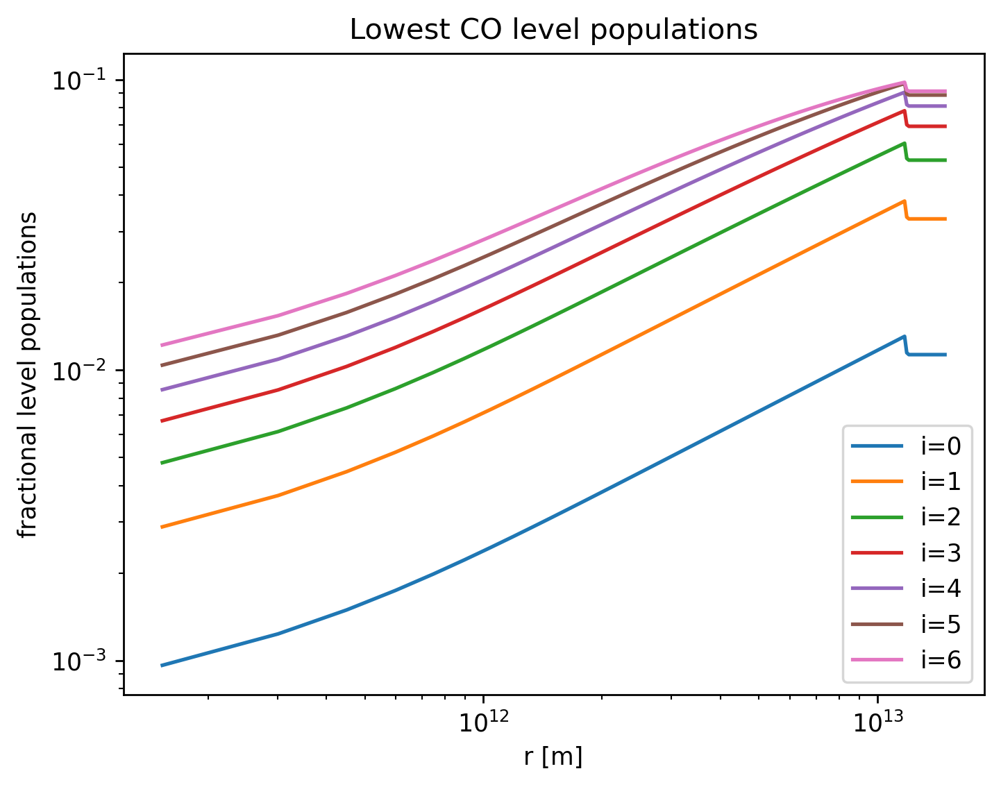
plt.figure(dpi=250)
plt.title('Lowest CO level populations')
for i in range(7):
    plt.plot(rs, pops[:,i]/ns, label=f'i={i}')

plt.xscale('log')
plt.yscale('log')
plt.ylabel('fractional level populations')
plt.xlabel('r [m]')
plt.legend()
[8]:
<matplotlib.legend.Legend at 0x7fc8682b3940>
Make synthetic observations
Now we can make synthetic observations of the model.
[9]:
fcen = model.lines.lineProducingSpecies[0].linedata.frequency[0]
vpix = 25   # velocity pixel size [m/s]
dd   = vpix * (model.parameters.nfreqs()-1)/2 / magritte.CC
fmin = fcen - fcen*dd
fmax = fcen + fcen*dd

model.compute_spectral_discretisation (fmin, fmax)
model.compute_image (model.parameters.hnrays()-1)

r = np.array(model.images[-1].ImX)
I = np.array(model.images[-1].I)
v = np.array(model.radiation.frequencies.nu)[0]
Computing spectral discretisation...
Computing image...
[10]:
import ipywidgets as widgets
from astropy import units
[11]:
def plot(p):
    plt.figure(dpi=150)
    plt.plot((v/fcen-1)*magritte.CC / 1000, I[p] - tools.I_CMB(v))
    plt.title(f'radius = {r[p]/(1.0*units.au).si.value:.0f} au')
    plt.xlabel('frequency [km/s]')
    plt.ylabel('intensity [W/m$^2$]')
widgets.interact(plot, p=(0, npoints-2))
[11]:
<function __main__.plot(p)>
(The plot is only interactive in a live notebook.)