1D AMRVAC

We create a Magritte model from a snapshot of 1D AMRVAC hydrodynamics simulation. The hydro model was kindly provided by Jan Bolte. Currently, the AMRVAC binary files can not yet be used directly to extract the snapshot data. Hence we use the corresponding .vtu files.

Setup

Import the required functionalty.

import magritte.setup    as setup                 # Model setup
import magritte.core     as magritte              # Core functionality
import numpy             as np                    # Data structures
import matplotlib.pyplot as plt                   # Plotting
import vtk                                        # Reading the model
import os

from tqdm                   import tqdm           # Progress bars
from astropy                import constants      # Unit conversions
from vtk.util.numpy_support import vtk_to_numpy   # Converting data

Define a working directory (you will have to change this; it must be an absolute path).

wdir = "/lhome/thomasc/Magritte-examples/AMRVAC_1D/"

Create the working directory.

!mkdir -p $wdir

Define file names.

input_file = os.path.join(wdir, 'model_AMRVAC_1D.vtu' )   # AMRVAC snapshot
model_file = os.path.join(wdir, 'model_AMRVAC_1D.hdf5')   # Resulting Magritte model
lamda_file = os.path.join(wdir, 'co.txt'              )   # Line data file

We use a snapshot and data file that can be downloaded with the following links.

input_link = "https://owncloud.ster.kuleuven.be/index.php/s/NpPG88x5LCbaZNC/download"
lamda_link = "https://home.strw.leidenuniv.nl/~moldata/datafiles/co.dat"

Dowload the snapshot and the linedata (%%capture is just used to suppress the output).

%%capture
!wget $input_link --output-document $input_file
!wget $lamda_link --output-document $lamda_file

Extract data

The script below extracts the required data from the snapshot .vtu file.

# Create a vtk reader to read the AMRVAC file and extract its contents.
reader = vtk.vtkXMLUnstructuredGridReader()
reader.SetFileName(input_file)
reader.Update()

# Extract the grid output
grid = reader.GetOutput()

# Extract the number of cells
ncells = grid.GetNumberOfCells()

# Extract cell data
cellData = grid.GetCellData()
for i in tqdm(range(cellData.GetNumberOfArrays())):
    array = cellData.GetArray(i)
    if (array.GetName() == 'rho'):
        rho = vtk_to_numpy(array)
    if (array.GetName() == 'temperature'):
        tmp = vtk_to_numpy(array)
    if (array.GetName() == 'v1'):
        v_x = vtk_to_numpy(array)

# Convert rho (total density) to abundances
nH2 = rho * 1.0e+6 * constants.N_A.si.value / 2.02
nCO = nH2 * 1.0e-4

# Convenience arrays
zeros = np.zeros(ncells)
ones  = np.ones (ncells)

# Since it is a 1D model there is no y or z data.
v_y = v_z = zeros

# Convert to fractions of the speed of light
velocity = np.array((v_x, v_y, v_z)).transpose() / constants.c.cgs.value

# Define turbulence at 150 m/s
trb = (150.0/constants.c.si.value)**2 * ones

# Extract cell centres to use as positions of the Magritte points.
centres = []
for c in tqdm(range(ncells)):
    cell = grid.GetCell(c)
    centre = np.zeros(3)
    for i in range(2):
        centre = centre + np.array(cell.GetPoints().GetPoint(i))
    centre = 0.5 * centre
    centres.append(centre)
centres  = np.array(centres)
centres *= 1.0e-2   # convert [cm] to [m]

# Define AMRVAC cell centres as Magritte point positions
position = centres

100%|███████████████████████████████████████| 85/85 [00:00<00:00, 346468.26it/s]
100%|███████████████████████████████████| 2000/2000 [00:00<00:00, 220677.35it/s]

Downsample the data by a factor 20. (Check whether this is a reasonable approximation for your radiative transfer model!)

reduction_factor = 20

position = position[::reduction_factor]
velocity = velocity[::reduction_factor]
nCO      = nCO     [::reduction_factor]
nH2      = nH2     [::reduction_factor]
tmp      = tmp     [::reduction_factor]
trb      = trb     [::reduction_factor]
zeros    = zeros   [::reduction_factor]
ones     = ones    [::reduction_factor]

ncells = len(position)

Create model

Now all data is read, we can use it to construct a Magritte model.

model = magritte.Model ()                              # Create model object

model.parameters.set_model_name         (model_file)   # Magritte model file
model.parameters.set_spherical_symmetry (True)         # Assume spherical symmetry
model.parameters.set_dimension          (1)            # Spherical symmetry is 1D
model.parameters.set_npoints            (ncells)       # Number of points
model.parameters.set_nrays              (50)           # Number of rays
model.parameters.set_nspecs             (3)            # Number of species (min. 5)
model.parameters.set_nlspecs            (1)            # Number of line species
model.parameters.set_nquads             (11)           # Number of quadrature points

model.geometry.points.position.set (position)
model.geometry.points.velocity.set (velocity)

model.chemistry.species.abundance = np.array((nCO, nH2, zeros)).T
model.chemistry.species.symbol    = ['CO', 'H2', 'e-']

model.thermodynamics.temperature.gas  .set(tmp)
model.thermodynamics.turbulence.vturb2.set(trb)

model = setup.set_Delaunay_neighbor_lists  (model)
model = setup.set_Delaunay_boundary        (model)
model = setup.set_boundary_condition_CMB   (model)
model = setup.set_uniform_rays             (model)
model = setup.set_linedata_from_LAMDA_file (model, lamda_file)
model = setup.set_quadrature               (model)

model.write()

Writing parameters...
Writing points...
Writing rays...
Writing boundary...
Writing chemistry...
Writing species...
Writing thermodynamics...
Writing temperature...
Writing turbulence...
Writing lines...
Writing lineProducingSpecies...
Writing linedata...
ncolpoar = 2
--- colpoar = 0
Writing collisionPartner...
(l, c) = 0, 0
--- colpoar = 1
Writing collisionPartner...
(l, c) = 0, 1
Writing quadrature...
Writing populations...
Writing radiation...
Writing frequencies...

Plot model

The data can be extracted from the Magritte model by casting it into numpy arrays.

position  = np.array(model.geometry.points.position)
velocity  = np.array(model.geometry.points.velocity)
abundance = np.array(model.chemistry.species.abundance)

rs  = np.linalg.norm(position, axis=1)
vs  = np.linalg.norm(velocity, axis=1)
nCO = abundance[:,1]

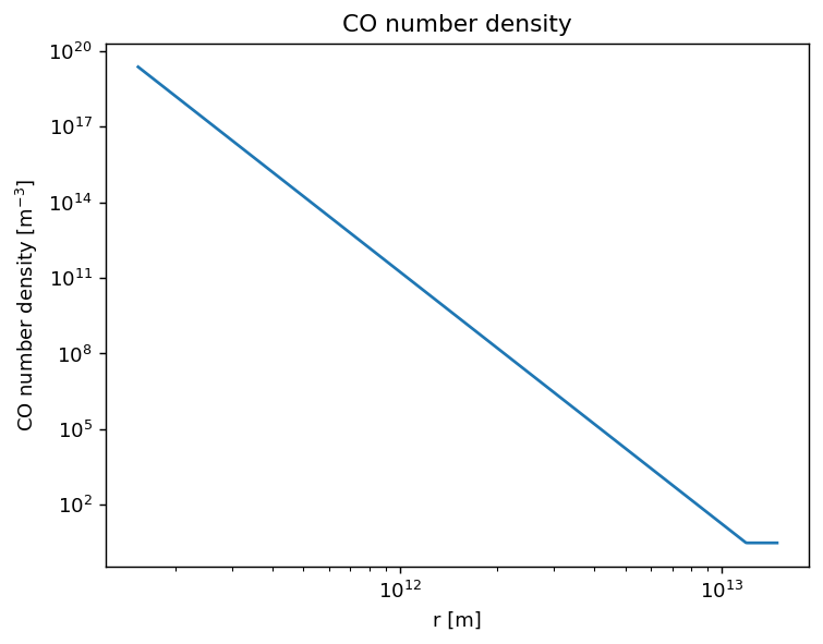
Plot of the CO number density.

plt.figure(dpi=130)
plt.title('CO number density')
plt.plot(rs, nCO)
plt.xscale('log')
plt.yscale('log')
plt.xlabel(r'r [m]')
plt.ylabel(r'CO number density [m$^{-3}$]')

Text(0, 0.5, 'CO number density [m$^{-3}$]')

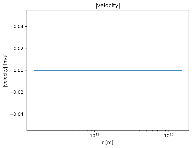
Plot of the lengths of the velocity vectors.

plt.figure(dpi=130)
plt.title('|velocity|')
plt.plot(rs, vs*magritte.CC)
plt.xscale('log')
plt.xlabel(r'r [m]')
plt.ylabel(r'|velocity| [m/s]')

Text(0, 0.5, '|velocity| [m/s]')